FREE Excel Tips Newsletter from TheExcelAddict.com Subscribe here to get more tips like this every week October 13, 2016   Hi fellow Excel Addict, In today's 'Excel in Minutes' tip I will be showing you how to 'View Data From Separate Areas of the Same Worksheet at the Same Time'. I hope you find it helpful. If you missed my 'Excel in Seconds' newsletter from Tuesday, I showed you how to 'Adjust A Range of Numbers By A Specific Amount Or Percentage'. You can read that tip here. I hope you have a great week and keep on Excelling, Francis Hayes (The Excel Addict) Email:  fhayes[AT]TheExcelAddict.com   If you missed my last newsletter, you can click here to view it online.   TheExcelAddict.com Quote of the Day "I could be another fool, or an exception to the rule." -- Elliott Smith --   If you have a favourite quote, send it to me and I may post it in my newsletter. View Data From Separate Areas of the Same Worksheet at the Same Time Most of our worksheets have data in one area that is dependent on data in another area. When you need to compare different parts of a large worksheet or see how changing data in one part affects the results in another part, it can be frustrating scrolling back and forth. Thankfully, Excel has a feature called split screen that allows you to easily view data from separate areas of the same worksheet at the same time. This split screen feature allows you to split one worksheet into two or four separate panes which then can be scrolled independently. Most commonly, Excel users use this feature to split a window into panes for comparing the contents of columns in separate parts of a worksheet. For example, you may want to compare the contents of column H with the contents of column Z. The same can be done for comparing distant rows as well. The big difference between Split screen and Freeze Panes is that with Freeze Panes, the topmost rows or leftmost panes are frozen, so you cannot scroll those sections. 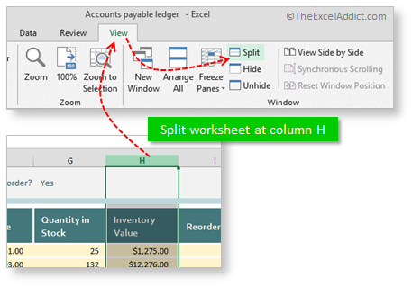Comparing distant columns 1) Click on a column heading (letter); 2) From the View tab click the Split command in the Window group. The window will be divided into two panes, each with its own horizontal scroll bar. In earlier versions of Excel (pre-2013), there is a 'split bar' located just left of the horizontal scroll bar. To split a worksheet into two panes (left and right), drag the split bar until the window is split as you want it.   3) You can use the horizontal scroll bar in each pane to bring the desired columns into view.  You can now use to vertical scroll bar to synchronously scroll up and down to view related data in both panes. To remove the split screen, drag the split bar (between column G and J in the example above) to the right edge of the screen or you can simply click Split on the View Ribbon tab. Compare distant rows 1) Click on a row heading (number); 2) From the View tab click the Split command in the Window group. The window will be divided into two panes, each with its own vertical scroll bar. In earlier versions of Excel (pre-2013), there is a 'split bar' located just above the vertical scroll bar. To split a worksheet into two panes (top and bottom), drag the split bar until the window is split as you want it. 3) You can use the vertical scroll bar in each pane to bring the desired rows into view.  You can now use to horizontal scroll bar to synchronously scroll right and left to view related data in both panes. To remove the split screen, drag the split bar (between rows 14 and 34 in the example above) to the top edge of the screen or you can simply click Split on the View Ribbon tab. 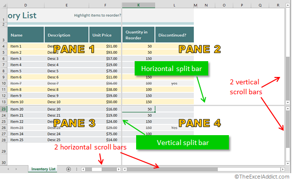Splitting your worksheet into four panes Similar to the above, you can also split your worksheet into four panes which allows you to view four different parts of a worksheet on the same screen. Start by selecting a cell at the intersection of where you want the split and clicking View, Split. Once the window has been split, you can drag the split bars to adjust the size of the panes. However, you cannot resize or scroll the columns in vertical panes (e.g. Pane 1 and 3 or Pane 2 and 4) independently and you cannot resize or scroll the rows in horizontal panes (e.g. Pane 1 and 2 or Pane 3 and 4) independently. To remove both split screens, click Split on the View tab. Alternatively, you can drag the vertical split bar (between columns F and K in the example above) to the left edge of the screen and drag the horizontal split bar (between rows 13 and 23 in the example above) to the top edge of the screen. FREE Excel Tips Newsletter from TheExcelAddict.com Subscribe here to get more tips like this every week Disclosure: Some of the resources I recommend on my website and in my newsletter pay me a small referral commission if you purchase from them through links on my website or using my referral code. This helps offset the costs of my website. I've worked long and hard to build up my reputation online over the past 10 years as someone who provides exceptional value to my readers. So I'm not willing to risk that. As you know, I don’t just recommend anything. It has to be of outstanding quality and value. If you are EVER not completely satisfied with anything I recommend, please let me know and you will get your money...GUARANTEED. You can't lose.

"Spreadsheets Tips From An Excel Addict" is a weekly publication of TheExcelAddict.com. Copyright Francis J. Hayes All Rights Reserved. 8 Lexington Place, Conception Bay South, Newfoundland, Canada, A1X 6A2 Phone: 709-834-4630