 |
|
| TheExcelAddict.com | |
| November 12, 2020 |
|
| Hi fellow Excel Addict, | |
Thanks for
joining me today for another 'Excel in Minutes' tip. All Remembrance Day parades in Canada (and I assume elsewhere) were cancelled to the public this year but I was fortunate to witness a young girl in our neighbourhood mark the 'eleventh hour of the eleventh day of the eleventh month' by playing "The Last Post" followed by two minutes of silence. I hope you will find today's 'Excel in Minutes' tip helpful. If you do, please help share my newsletter on your social media accounts and with your colleagues or any other Excel users you know who want to get smarter with Excel. Have a great day, keep safe and keep on Excelling, Francis Hayes (The Excel Addict) Email: fhayes[AT]TheExcelAddict.com |
|
|
|
|
|
|
|
| Missed my last newsletter? | |
Click Here to View it Online |
|
Having a positive attitude can help us in difficult times. I hope today's quote will help you foster a positive attitude today. Quote of the Day "Democracy is based upon empathy and the recognition that some decisions are solely for the community's benefit without regard to one's own narrow self-interest." -- John Hickenlooper -- |
|
|
If you have a favourite quote, send it to me
and I may post it in my newsletter.
|
|
THIS WEEK'S 'EXCEL IN MINUTES' TIP |
|
Look Up The Last Instance Of A Value In One Column And Return A Related Value from Another Column |
|
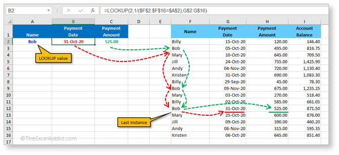
This week an Excel Addict subscriber asked me how she could return the last Payment Date and Payment Amount for a specific payee's Name in a table. As with many things in Excel, there are often multiple ways to do this but I'd like to show you one that I suggested.  This is the formula I used to find the Payment Date related to the last instance of the name Bob (i.e. value input into cell A2). =LOOKUP(2,1/($F$2:$F$16=$A$2),$G$2:$G$16)
=LOOKUP(lookup_value,
lookup_range, result_range)
The LOOKUP function uses 'approximate matching' to look up a lookup_value in a one-column (or one-row) lookup_range and returns a value from a corresponding one-column (or one-row) result_range. This formula takes advantage of the 'approximate matching' feature of the LOOKUP function to help solve this problem. The Lookup Value The first argument in the LOOKUP function is the lookup_value. Here Im using a value of 2. Ill explain why later. The Lookup Range The second argument in the LOOKUP function is the lookup_range. Here Ive used $F$2:$F$16=$A$2 as the lookup range. To see how this works, highlight $F$2:$F$16 in the formula bar...   Next highlight $A$2 in the formula bar and press the F9 key and youll see the lookup_value.  Next, the values {"Billy";"Bob";"Mary";"Jill";"Andy";"Kristen";"Billy";"Bob";"Mary";"Billy";"Bob"; "Mary";"Jill";"Andy";"Kristen"} are matched with the lookup_value "Bob" and evaluate to either TRUE or FALSE.  Next in this formula, 1 is divided by each of those TRUE and FALSE values.  In Excel, TRUE is equal to 1 and FALSE is equal to 0. So, when 1 is divided by TRUE you get 1 (i.e. 1/1) and when 1 is divided by FALSE you get a #DIV/0! error (i.e. 1/0). The result is an array of 15 values that are used as the lookup_range for this LOOKUP function.  The purpose of using 2 as the lookup_value is to use a value that is greater than any value in the lookup_range, forcing it to search the entire lookup_range without finding a matching value. Since the LOOKUP function uses approximate matching and scans the entire lookup_range for a match to the lookup_value (i.e. 2), it returns the position of the last value that is the next largest value (i.e. 1) which is lower than the lookup_value. In this example, that value (i.e. the last 1) is found in the 11th position. The Result Range To finish this off, let's look at the third argument of the LOOKUP function the result_range. If you highlight the result_range in the formula bar and press the F9 key, you will see a list of 15 values. Although, in the worksheet the result_range contains dates, in formulas, Excel shows dates as their decimal equivalents (e.g. 44135 = October 31, 2020).  In the final step, the 11th position that was found in the lookup_range is used to return the 11th position from the result_range. So, now we know the Last Payment Date for Bob was October 31, 2020.  To find a corresponding value from another column (e.g. Payment Amount), simply adjust the column references for the result_range. =LOOKUP(2,1/($F$2:$F$16=$A$2),$G$2:$G$16)
to
=LOOKUP(2,1/($F$2:$F$16=$A$2),H$2:H$16)
|
|
|
|
|
|
|
|
 |
|
|
|
|
| Disclosure: Some of the resources I recommend on my website and in my newsletter pay me a small referral commission if you purchase from them through links on my website or using my referral code. This helps offset the costs of my website. I've worked long and hard to build up my reputation online over the past 16 years as someone who provides exceptional value to my readers. So I'm not willing to risk that. As you know, I dont just recommend anything. It has to be of outstanding quality and value. If you are EVER not completely satisfied with anything I recommend, please let me know and you will get your money...GUARANTEED. You can't lose. | |
