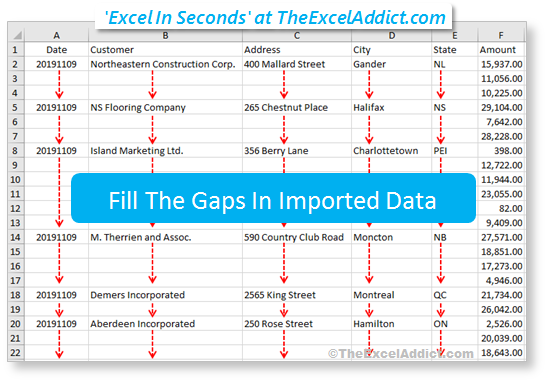
When you bring data into Excel from another source (or copy data from a Pivot Table), oftentimes some of the cells are left blank, indicating a repeating value from above. This may make the information easier to read but it also means that you cannot use many of Excel's best features, such as filtering, subtotaling and Pivot Tables to manipulate this data.


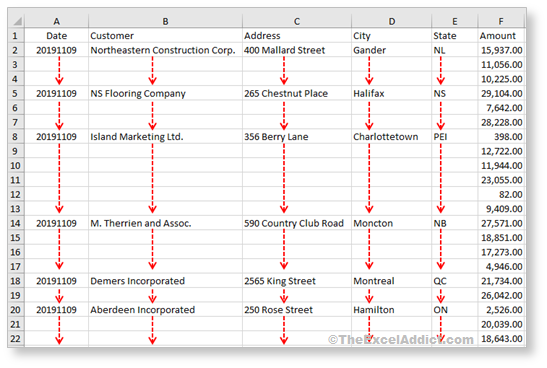
If you have only a small amount of data, you can simply fill down (CTRL+D) or Copy and Paste the values for each blank section. However, when you are dealing with hundreds or even thousands of records, those methods are not practical.

Today I want to show you a 'fairly simple' process to help you complete this task in less than a minute, regardless of how many records you are dealing with.

In this example we are going to fill all the gaps in columns A to E.

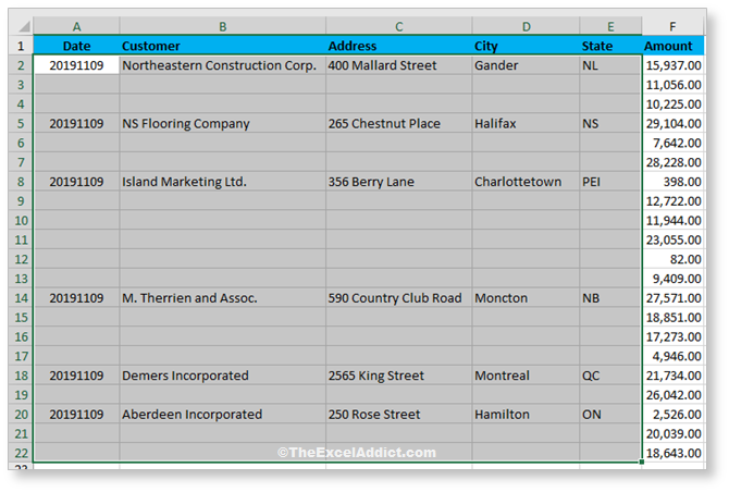
1) Select all of the data, both blank and non-blank cells, in a single range (e.g. A1:E22);


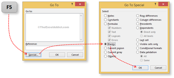
2) Press the F5 key on your keyboard and click the Special... button in the 'Go To' dialog. Then select the Blanks option in the 'Go To Special' dialog and click OK;


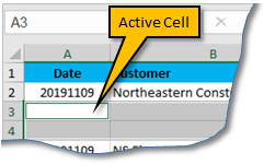
3) Now, only the blank cells are selected;


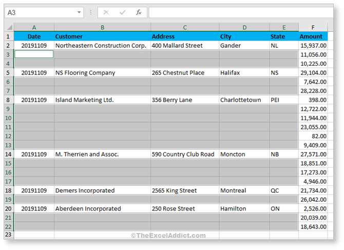
Notice that the 'Active Cell' is now A3.


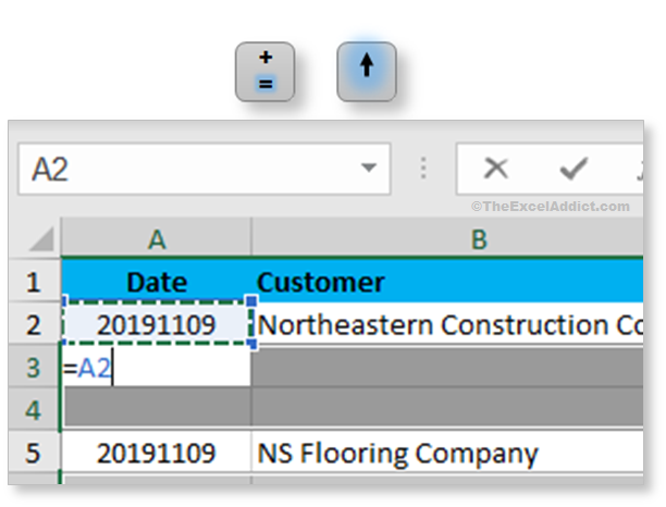
4) Next, press the equals sign (=) key, then press the 'up arrow' key once. This will create a formula reference to the cell immediately above the Active Cell;


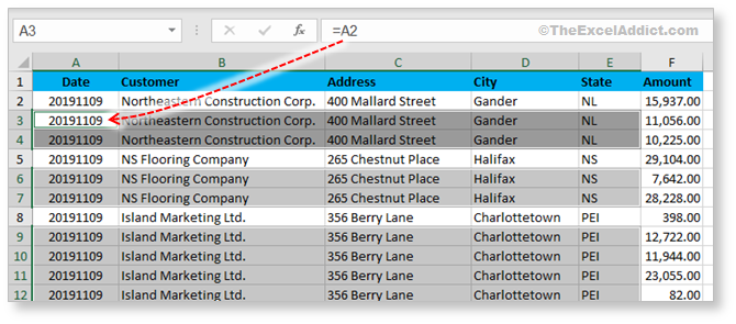
5) Now hold down the CTRL key and press Enter. This will fill each of the selected (blank) cells with a formula (e.g. =A2) that references the cell above itself;


6) Next, re-select the entire data range again and move your mouse pointer to the edge of the selected range until it changes to a 4-headed arrow (see image below);

7) Press the right mouse button and drag the cells a little to the right, BUT DON'T RELEASE THE MOUSE BUTTON. Still holding down the mouse button, drag back to the original location and release the button (see image below).

8) Click the 'Copy Here as Values Only' option from the menu that pops up to replace the formulas with fixed values.


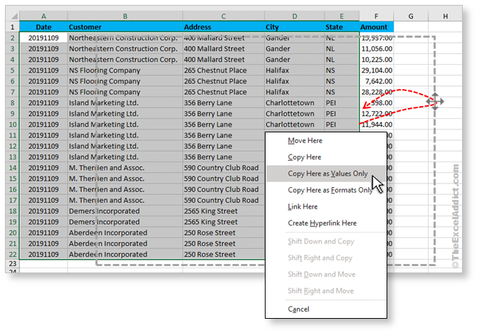
Now all of the previously empty cells are filled with the values from above and your data is ready for sorting, filtering, subtotaling, etc...;

Go ahead. Open this practice file and try it for yourself now... It's easy.